Workflow 1: Define Gating Strategy and Polygon Gates
Source:vignettes/workflow_1.Rmd
workflow_1.RmdThere are two basic scenarios when using flowdex that
further define the appropriate workflow:
Gating strategy and polygon gates are not yet defined.
Here, the focus is on establishing the gating strategy and manually drawing the polygon gates.Gating strategy and polygon gates are already defined.
Here, the focus is on using the previously established gating strategy to extract fluorescence distributions, visualise them and export them to file. All this (except visualisation) is conveniently done viaflowdexit(). Look at Quickstart for an immediate example.
Workflow 1
If not already done, set up the tutorial data as described in Get Started.
The next step after data
acquisition is to visualize the raw-counts, to decide which sample
to use for drawing the gate, and then to manually draw the polygon
gate(s) and safe them for later use.
Each row in the gating strategy file defines a single gate along with
its polygon gate definition. Gates can be nested or ‘standalone’.
If not already done, set the working directory to the ‘tap_water_home’ folder:
Read in fcs Files and Make Gating Set
Before drawing a polygon gate on a single sample, we have to read in some fcs files and produce the gating set.
gsAll <- makeGatingSet()
#> Reading in fcs files... ok.
#> Producing gating set... Applying fjbiexp transformation... ok.
If everything was left at the default, this will read in all 108
fcs-files contained in the folder ‘fcsFiles’.
For the purpose of this demonstration we will restrict the fcs files to
be read in to a lower number by defining a filename pattern: Only fcs
files with matching pattern will be read in.
gsRed <- makeGatingSet(patt="GPos_T6_th2")
#> Reading in fcs files... ok.
#> Producing gating set... Applying fjbiexp transformation... ok.
gsRed
#> A GatingSet of class 'GatingSet' with 6 samples:
#>
#>   Index             SampleNames
#> 1     1 N_na_GPos_T6_th2_b1.fcs
#> 2     2 N_na_GPos_T6_th2_b2.fcs
#> 3     3 N_na_GPos_T6_th2_b3.fcs
#> 4     4 N_na_GPos_T6_th2_b4.fcs
#> 5     5 N_na_GPos_T6_th2_b5.fcs
#> 6     6 N_na_GPos_T6_th2_b6.fcs
#>
#>
#> The following 10 channels are available:
#> FSC.A    SSC.A    FITC.A    PE.A    PerCP.A    PE.Cy7.A    APC.A    APC.Cy7.A    V450.A    V500.A
Note the printout of the samples contained in the gating set and of
the available channels.
Only fcs files from the experiment group from day 6 (second third,
i.e. 6 beakers) were read in.
We can now use this reduced gating set to visualise the raw fcs data by specifying the channel we want for the x and for the y axis:
plotgates(gsRed, toPdf = FALSE, x="FITC.A", y="PerCP.A")
#> Coordinate system already present. Adding new coordinate system, which will replace the existing one.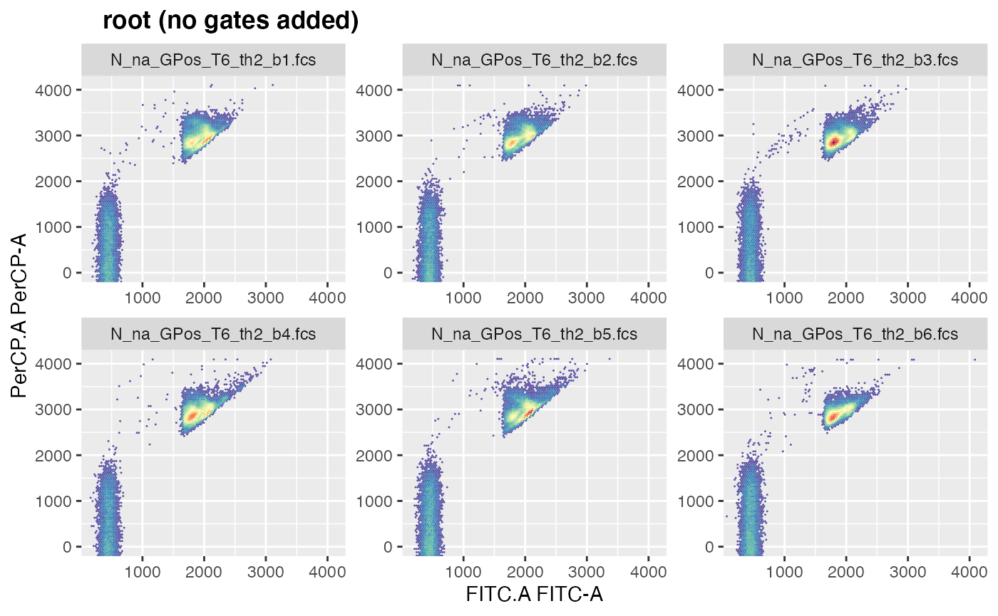
Manually Draw Polygon Gate
All 6 samples seem to have a good representation of our desired
population, the stained bacteria.
Lets assume we choose beaker ‘GPos_T6_th2_b4’, which is the 4th sample
in this gating set, as sample to manually draw the polygon gate on:
drawGate(gsRed, flf=4, gn="root", pggId="BactStainV1", channels=".")
# point and click to draw a polygon gate around the population of interest;gnis the name of the gate we want to use to display data. As no gates are yet defined let alone added to the gating set, we leave that at the default ‘root’.pggIdspecifies the name the new polygon gate should be saved under. If left at the default, ‘polyGate’ will be used.channelsis specifying which channels we want to be displayed on the x and y axis. Defaults to ‘c(“FITC.A”, “PerCP.A”)’.The lines displayed in the graphic have their origin in the
bndargument, defining the boundaries to be displayed.
(All default values can be easily changed in the ‘flowdex_settings.R’ file located at ‘~/desktop/flowdex_SH’.)
If you are not satisfied with the polygon gate definition, you can draw it again while simultaneously displaying an other (the old) gate:
drawGate(gsRed, flf=4, gn="root", pggId="BactStainV1", show="BactStainV1")
# point and click to draw an improved polygon gate around the population of interest
Polygon gate definitions get automatically saved under the specified name in the folder ‘gating’.
You can leave the gate definition of ‘BactStainV1’ as you were drawing it, or you can copy the gate definition that was originally drawn for this project:
from <- paste0(td, "/flowdex_tutorial/gating/BactStainV1")
to <- paste0(td, "/tap_water_home/gating")
file.copy(from, to, overwrite = TRUE)
#> [1] TRUE
And now visualize the gate, this time without using the locator:
drawGate(gsRed, flf=4, gn="root", show="BactStainV1", useLoc = FALSE) 
Write Gating Strategy
For each gate that you want to apply to your gating set, there has to be one row in the gating strategy file. Now copy the template for the gating strategy file into the experiment home folder:
from <- paste0(td, "/tap_water_home/templates/gateStrat.xlsx")
to <- paste0(td, "/tap_water_home/gating")
file.copy(from, to)
#> [1] TRUE
Open the copied file. For every gate, i.e. every row, all 8 fields have to filled in.
The ‘GateName’ is, obviously, the name of the gate. Short names recommended.
‘Parent’ is the name of the parent-gate, i.e. the gate where the data are coming from. In the first row, this has to be ‘root’.
‘GateOnX’ and GateOnY’ define the channels to be used for that gate in the x and y axis.
‘GateDefinition’ is the name of the polygon gate manually drawn in the previous step.
‘extractOn’ defines on which channel, i.e. along which axis the fluorescence data should be extracted. Must be either the channel used for the x axis or the channel used for the y axis.
‘minRange’ and ‘maxRange’ define the lower and upper limit of the channel where data are extracted. It is recommended that gate definitions do not go beyond these limits. To facilitate this, use the boundary
bndargument indrawGate().‘keepData’ is denoting whether the data from this gate are to be kept or not. Set this field to FALSE when the data of this gate are not of interest and it is merely used to prepare the data for an other, a nested gate. There has to be at least one field in ‘keepData’ set to TRUE.
The column names must not be changed.
For the example at hand, fill in the gating strategy file as follows:
GateName: DNA+
Parent: foot
GateOnX: FITC.A
GateOnY: PerCP.A
GateDefinition: BactStainV1
extractOn: FITC.A
minRange: 1250
maxRange: 4000
keepData: TRUE
Or copy the already filled out gating strategy file defining the gate ‘DNA+’ with its polygon gate definition ‘BactStainV1’ from the tutorial folder:
from <- paste0(td, "/flowdex_tutorial/gating/gateStrat.xlsx")
to <- paste0(td, "/tap_water_home/gating")
file.copy(from, to, overwrite=TRUE)
#> [1] TRUE
Now everything should be ready to apply the gating strategy to the gating set:
gsRed_ga <- addGates(gsRed) # gsRed was created above
#> Gating: (1 gate)
#> done!
flowWorkspace::plot(gsRed_ga) # to view the gate hierarchy 
plotgates(gsRed_ga, toPdf = FALSE) # to view the gated data
#> Coordinate system already present. Adding new coordinate system, which will replace the existing one.
#> .Draw Gate, Add to Gating Strategy, Add Gate to Gating Set – and Repeat
When more than one gate should be defined in the gating strategy, the circle of
drawing the gate on a single sample,
adding that gate to the gating strategy (file), and
adding that gate to the gating set (object)
is repeated for every gate that should be applied to the fcs data.
In the next iteration, i.e. when for example a second gate within the data from the first gate should be defined, one would call:
drawGate(gsRed_ga, flf=5, gn="DNA+", pggId="pg2", channels = c("FITC.A", "SSC.A"))
# point and click to draw a polygon gate around the population of interest
Then go modify the gating strategy file (extracting along SSC is probably not meaningful, but just to show that it can be done):
GateName: FooGate
Parent: DNA+
GateOnX: FITC.A
GateOnY: SSC.A
GateDefinition: pg2
extractOn: SSC.A
minRange: 0
maxRange: 4000
keepData: TRUE
gsRed_ga <- addGates(gsRed_ga) # add the gate to the gating set Repeat these three steps to define any set of possibly nested gates. You can always view the gating hierarchy and the gated data via:
flowWorkspace::plot(gsRed_ga) # to view the gating hierarchy
plotgates(gsRed_ga, toPdf = F) # to view the gated data
Use a Ready-Made Example for Nested Gates
Copy a ready made example for a gating strategy holding more than one gate from the tutorial folder in the experiment home folder
from <- list.files(paste0(td, "/flowdex_tutorial/gating"), full.names = TRUE)
to <- paste0(td, "/tap_water_home/gating")
file.copy(from, to, overwrite=TRUE) # this might overwrite the polygon gate definition you created above
#> [1] TRUE TRUE TRUE TRUE TRUE TRUE
and apply it to a gating set. For ease of demonstration, we will
again use a subset of the fcs files as above. Reading in the fcs files
and adding the gates can be conveniently done using
makeAddGatingSet():
# we are not using the default name for gating strategy any more:
gsRed2 <- makeAddGatingSet(patt="GPos_T6_th2", gateStrat = "gateStrat_2")
#> Reading in fcs files... ok.
#> Producing gating set... Applying fjbiexp transformation... ok.
#> Gating: (6 gates)
#> done!
flowWorkspace::plot(gsRed2) # to view the gating hierarchy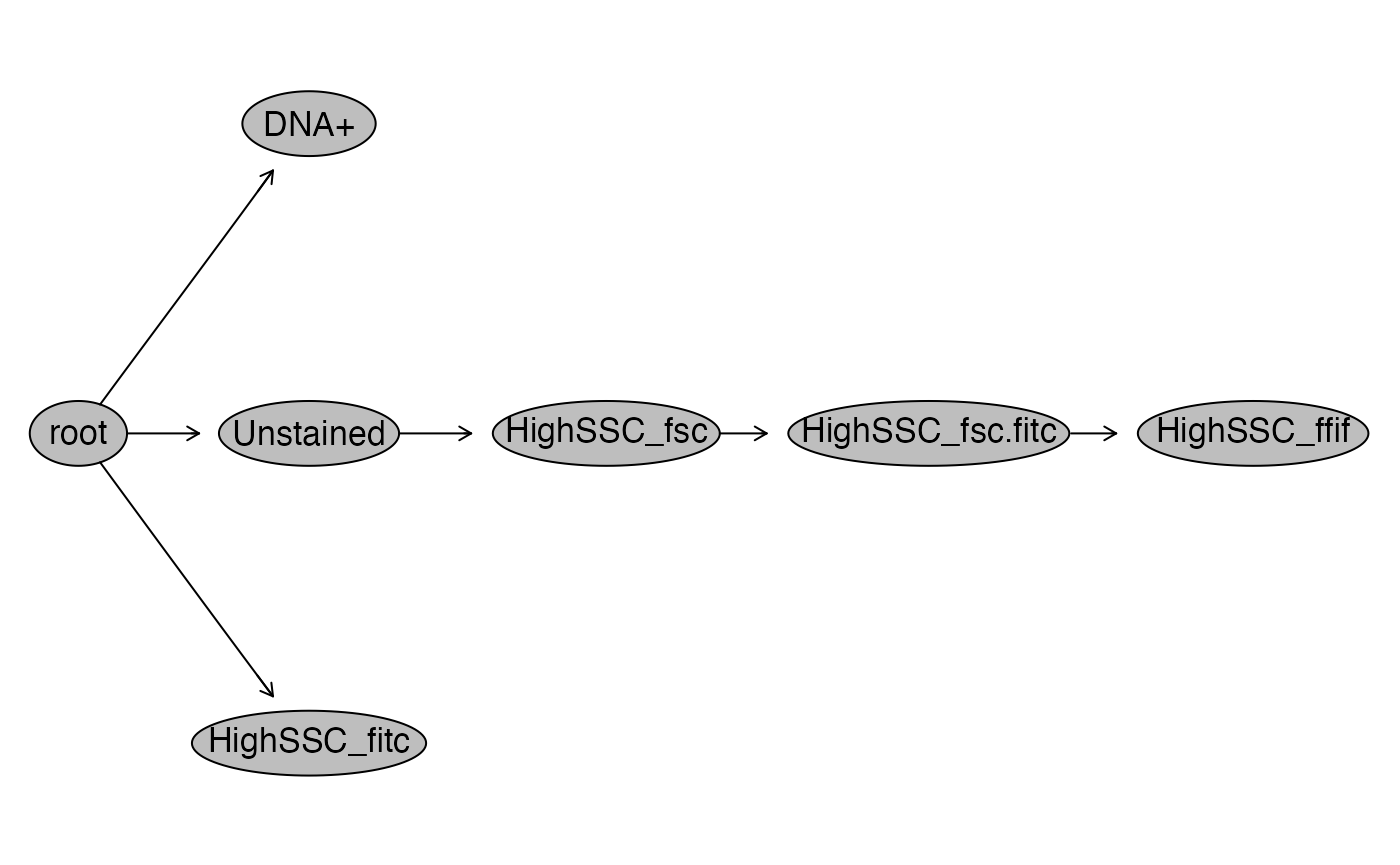
plotgates(gsRed2, toPdf = FALSE) # to view the gated data
#> Coordinate system already present. Adding new coordinate system, which will replace the existing one.
#> .....
#> Coordinate system already present. Adding new coordinate system, which will replace the existing one.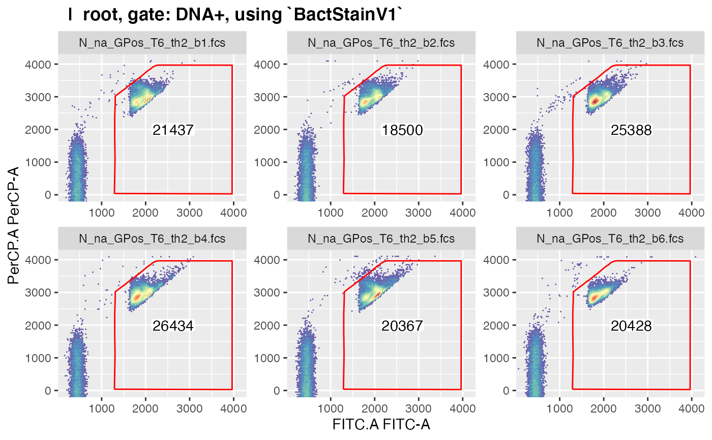
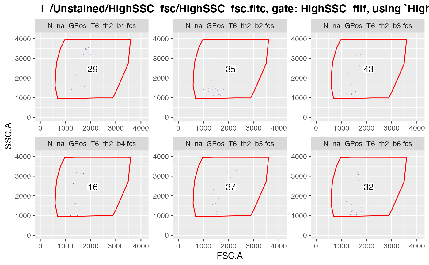
#> .Note that only those gated data get displayed in
plotgates() where the field ‘keepData’ in the gating
strategy file is set to ‘TRUE’.
(Admittedly, the practical value of this gating hierarchy is rather
non-existent, but it is merely for demonstrating the setup of nested
gates…)
Continue to Workflow 2.