If not already done, set up the tutorial data as described in Get Started and Workflow 2.
Set the working directory to ‘tap_water_home’:
Check and Repair fcs Files
As it also happened to the author, sometimes the FCM-machine seems to have written a kind of ‘faulty’ fcs file, resulting in the error message
The HEADER and the TEXT segment define different starting point ... to read the datawhen trying to add a gate to the previously read in fcs files.
Reading in those fcs files via
flowCore::read.FCS() was not the problem – at least in the
authors case.
After some testing it was concluded that the reason for that error
appears to lie in a multiplication of keywords in the afflicted fcs
files. Thus, the function checkRepairFcsFiles() was written
to remove all but one of each of the multiplied keywords.
checkRepairFcsFiles() is automatically executed whenever
fcs files are read in.
However, the default is to not repair the afflicted fcs
files, but to merely list the possibly erroneous files and to stop.
If so desired, checkRepairFcsFiles() can be called
manually in order to have more options: Multiple keywords can be viewed,
and it can be selected which one of the multiples of each keyword to
keep.
For the purpose of this demonstration, some fcs files provoking the error as described above are included in the tutorial dataset. First, copy the faulty fcs files to a folder in the experiment-home directory:
td <- tempdir()
from <- list.files(paste0(td, "/flowdex_tutorial/fcsF_E_rep"), full.names=TRUE)
to <- paste0(td, "/tap_water_home/fcsF_E_rep")
dir.create(to)
file.copy(from, to, overwrite=TRUE)
#> [1] TRUE TRUE TRUE
Now check for faulty fcs files:
checkRepairFcsFiles(fn="fcsF_E_rep")

#> The following 2 files from the folder 'fcsF_E_rep'
#> do have non-unique entries (all 2 fold) in their keywords:
#> N_na_GNeg_T6_th1_b2.fcs
#> N_na_GNeg_T6_th1_b3.fcs
#> Fehler: Consider setting 'fcsRepair' to TRUE.
#> CAVE: Original fcs files will then be overwritten.
We see that two files have multiplied keywords. Repair them by calling
checkRepairFcsFiles(fn="fcsF_E_rep", fcsRepair = TRUE, confirm = FALSE)
#>
#> The following 2 files from the folder 'fcsF_E_rep'
#> do have non-unique entries (all 2 fold) in their keywords:
#> N_na_GNeg_T6_th1_b2.fcs
#> N_na_GNeg_T6_th1_b3.fcs
#>
#> All except the last of each multiplied keyword were removed, and the original fcs file were overwritten.
#> (You can use 'checkRepairFcsFiles' directly and set 'showMultiples' to TRUE to display the multiplied keywords.)
# check again, all should be good now:
checkRepairFcsFiles(fn="fcsF_E_rep")
#> All fcs files in the folder 'fcsF_E_rep'
#> seem to be ok, i.e. do have only single entries in their keywords.
Please refer to checkRepairFcsFiles() for further
information on how to view multiplied keywords and how to select which
one of each multiple to keep.
Repair Sample ID and Volume Data
In case it happened that the volumetric measurement of a single
sample did not succeed, or that an erroneous sample-ID string was
provided in the sample-ID field of a single sample at the time of data
acquisition, there are two functions to remedy these issues:
repairVolumes() and repairSID().
Repair Volumes
First, copy some (manipulated) fcs files to a folder in the experiment-home directory:
from <- list.files(paste0(td, "/flowdex_tutorial/fcsF_E_vol_sid"), full.names=TRUE)
to <- paste0(td, "/tap_water_home/fcsF_E_vol_sid")
dir.create(to)
file.copy(from, to, overwrite=TRUE)
#> [1] TRUE TRUE TRUE TRUE
In order to repair missing volume data, call
# repairVolumes(fn = "fcsF_E_vol_sid", vol=1234567) # press enter to confirm, displays more information.
# (Not suitable for the vignette.)
#
repairVolumes(fn = "fcsF_E_vol_sid", vol=1234567, confirm=FALSE)
#> Reading in all fcs files in the folder `fcsF_E_vol_sid`... ok.
#> Re-writing volume data of 2 FCS files, using `1234567` to replace missing values.
#> .. ok.
# and check again:
repairVolumes(fn = "fcsF_E_vol_sid", vol=1234567) # all should be good
#> Reading in all fcs files in the folder `fcsF_E_vol_sid`... ok.
#> All volume values are present - no re-writing of fcs files will be performed.
Please note that when leaving confirm at its default
TRUE, more details regarding the fcs files to be repaired / re-written
to disc are displayed.
If you want to force all fcs files in a folder to
have the same volume data, you can set the argument
includeAll to TRUE:
repairVolumes(fn = "fcsF_E_vol_sid", vol=1010101, confirm=FALSE, includeAll = TRUE)
#> Reading in all fcs files in the folder `fcsF_E_vol_sid`... ok.
#> Re-writing volume data of 4 FCS files, using `1010101` to replace present or missing values.
#> .... ok.
Repair Sample ID
Assuming you repaired the volume data as described above, we can use the fcs files in the folder
‘fcsF_E_vol_sid’ to demonstrate how to repair a faulty sample ID.
It is more than likely that sometimes (e.g. in the long nights of data
acquisition because the FCM-machine is so occupied that you are driven
to the long hours after dark…) an erroneous sample ID character is
provided in the sample ID field of an individual sample at the time of
data acquisition (see the structured
ID string).repairSID() can be used to repair these faulty sample
IDs.
In the best case, a faulty sample ID comes to your attention because
the translation of element names via the dictionary does not work.
In the worst case, the element value is wrong. This only comes to your
attention when e.g. cross-referencing the sample names and the cyTags /
the sample IDs in the pData slot of the ‘fdmat’
object (as produced e.g. by flowdexit() —
if there are descriptive sample names…
To repair a faulty sample ID in a single fcs file, you first have to
read in all (or some; use argument patt) fcs files in a
folder; they come back as flowCore::flowSet().
Then this ‘flowSet’ is given again to the function
repairSID(), but now a sample name and its new sample ID
can be specified:
flowset <- repairSID(fn = "fcsF_E_vol_sid")
#
flowset@phenoData@data # very bad sample ID in the fourth sample
#>                          volume     btim
#> N_na_GNeg_T4_th1_b4.fcs 1010101 14:19:30
#> N_na_GNeg_T5_th3_b3.fcs 1010101 14:34:13
#> N_na_GPos_T5_th1_b1.fcs 1010101 14:43:57
#> N_na_GPos_T5_th1_b3.fcs 1010101 14:47:13
#>                                                                             sampleId
#> N_na_GNeg_T4_th1_b4.fcs tr: GNeg; Td: 4; wt: nativ; ap: no; th: th1; ha: ha1; bk: b4
#> N_na_GNeg_T5_th3_b3.fcs tr: GNeg; Td: 5; wt: nativ; ap: no; th: th3; ha: ha2; bk: b3
#> N_na_GPos_T5_th1_b1.fcs tr: GPos; Td: 5; wt: nativ; ap: no; th: th1; ha: ha1; bk: b1
#> N_na_GPos_T5_th1_b3.fcs                                 blablabla very bad sample ID
#>                                            name
#> N_na_GNeg_T4_th1_b4.fcs N_na_GNeg_T4_th1_b4.fcs
#> N_na_GNeg_T5_th3_b3.fcs N_na_GNeg_T5_th3_b3.fcs
#> N_na_GPos_T5_th1_b1.fcs N_na_GPos_T5_th1_b1.fcs
#> N_na_GPos_T5_th1_b3.fcs N_na_GPos_T5_th1_b3.fcs

#
# view the correct sample IDs of the other samples
# copy one of those correct sample IDs
# paste and modify it - it should be beaker #3:
nsid <- "tr: GPos; Td: 5; wt: nativ; ap: no; th: th1; ha: ha1; bk: b3"

#
# also copy and paste the sample name
sana <- "N_na_GPos_T5_th1_b3.fcs" # the  name of the sample having the faulty sample ID

#
# now put all together and write fcs file with correct sample ID back to disk
repairSID(fs=flowset, fn="fcsF_E_vol_sid", name=sana, newSID = nsid, confirm = FALSE)
#> `N_na_GPos_T5_th1_b3.fcs` has been rewritten with the modified sample ID.

#
# and check again:
flowset <- repairSID(fn = "fcsF_E_vol_sid")
flowset@phenoData@data # all is good
#>                          volume     btim
#> N_na_GNeg_T4_th1_b4.fcs 1010101 14:19:30
#> N_na_GNeg_T5_th3_b3.fcs 1010101 14:34:13
#> N_na_GPos_T5_th1_b1.fcs 1010101 14:43:57
#> N_na_GPos_T5_th1_b3.fcs 1010101 14:47:13
#>                                                                             sampleId
#> N_na_GNeg_T4_th1_b4.fcs tr: GNeg; Td: 4; wt: nativ; ap: no; th: th1; ha: ha1; bk: b4
#> N_na_GNeg_T5_th3_b3.fcs tr: GNeg; Td: 5; wt: nativ; ap: no; th: th3; ha: ha2; bk: b3
#> N_na_GPos_T5_th1_b1.fcs tr: GPos; Td: 5; wt: nativ; ap: no; th: th1; ha: ha1; bk: b1
#> N_na_GPos_T5_th1_b3.fcs tr: GPos; Td: 5; wt: nativ; ap: no; th: th1; ha: ha1; bk: b3
#>                                            name
#> N_na_GNeg_T4_th1_b4.fcs N_na_GNeg_T4_th1_b4.fcs
#> N_na_GNeg_T5_th3_b3.fcs N_na_GNeg_T5_th3_b3.fcs
#> N_na_GPos_T5_th1_b1.fcs N_na_GPos_T5_th1_b1.fcs
#> N_na_GPos_T5_th1_b3.fcs N_na_GPos_T5_th1_b3.fcs
Apply Bandpass Filter
Function applyBandpass() does exactly what it says – it
applies a bandpass-like filter to the fluorescence intensities stemming
from a single gate.
If not already done before, create an ‘fdmat’ object containing only a
small subset of the data:
fdmat_s <- flowdexit(patt = "T4_th1")
#> Reading in fcs files... ok.
#> Producing gating set... Applying fjbiexp transformation... ok.
#> Gating: (1 gate)
#> done!
#> DNA+: Extracting binned data on FITC.A (res=220) and recalc. to volume... ok.
#> Exporting data (1 gate) to xlsx...ok.
#> fdmat-object saved.
plotFlscDist(fdmat_s, toPdf = FALSE)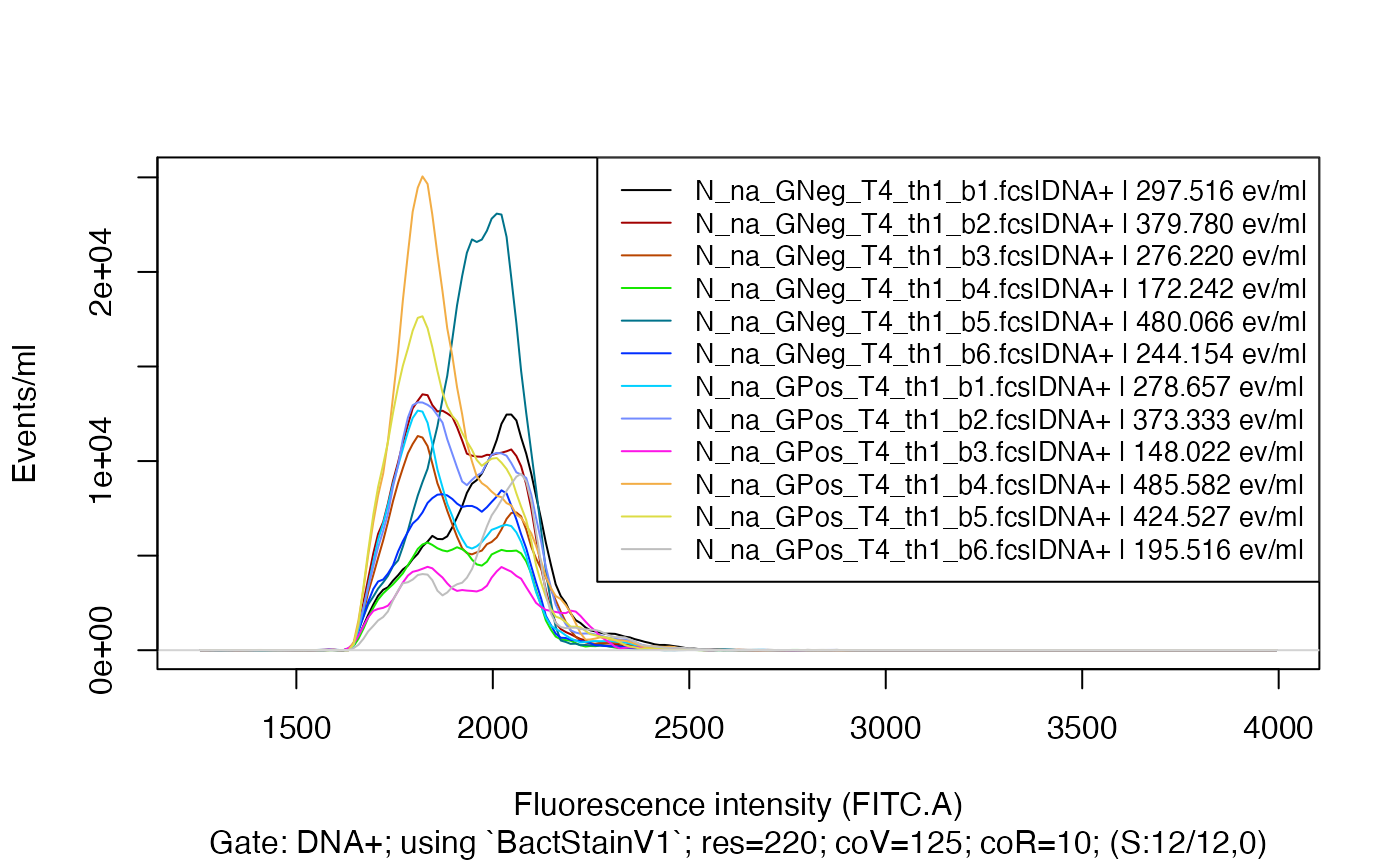
We see not much signal below the fluorescence intensity 1600 and
above 2400.
Lets apply a bandpass filter to our ‘fdmat’ object so that only those
fluorescence intensities between 1600 and 2400 remain:
fdmat_s_bp <- applyBandpass(fdmat_s, bandpass = c(1600, 2400))
fdmat_s[[1]] # compare
#> An object of class 'fdmat_single'
#> containing data from 12 samples in 219 fluorescence intensities from flsc1256 to flsc3994
#> derived from gate 'DNA+'.
#> original
#>                               flsc1256 flsc1269 flsc1281 flsc3969 flsc3981
#> N_na_GNeg_T4_th1_b1.fcs|DNA+ 0.0000000        0 0.000000        0        0
#> N_na_GNeg_T4_th1_b2.fcs|DNA+ 0.0000000        0 0.000000        0        0
#> N_na_GPos_T4_th1_b5.fcs|DNA+ 0.9221548        0 1.998002        0        0
#> N_na_GPos_T4_th1_b6.fcs|DNA+ 0.0000000        0 0.000000        0        0
#>                              flsc3994
#> N_na_GNeg_T4_th1_b1.fcs|DNA+        0
#> N_na_GNeg_T4_th1_b2.fcs|DNA+        0
#> N_na_GPos_T4_th1_b5.fcs|DNA+        0
#> N_na_GPos_T4_th1_b6.fcs|DNA+        0
#> (showing only the first and last columns and rows)
#>
#> Overall data for events per volume unit:
#>                         events_ml mean is_filtered events_ml_orig
#> N_na_GNeg_T4_th1_b1.fcs    297516 1985       FALSE         297516
#> N_na_GNeg_T4_th1_b2.fcs    379780 1913       FALSE         379780
#> N_na_GNeg_T4_th1_b3.fcs    276220 1913       FALSE         276220
#> N_na_GNeg_T4_th1_b4.fcs    172242 1925       FALSE         172242
#> N_na_GNeg_T4_th1_b5.fcs    480066 1954       FALSE         480066
#> N_na_GNeg_T4_th1_b6.fcs    244154 1923       FALSE         244154
#> N_na_GPos_T4_th1_b1.fcs    278657 1893       FALSE         278657
#> N_na_GPos_T4_th1_b2.fcs    373333 1923       FALSE         373333
#> N_na_GPos_T4_th1_b3.fcs    148022 1954       FALSE         148022
#> N_na_GPos_T4_th1_b4.fcs    485582 1889       FALSE         485582
#> N_na_GPos_T4_th1_b5.fcs    424527 1895       FALSE         424527
#> N_na_GPos_T4_th1_b6.fcs    195516 1993       FALSE         195516
fdmat_s_bp[[1]] #
#> An object of class 'fdmat_single'
#> containing data from 12 samples in 64 fluorescence intensities from flsc1608 to flsc2399
#> derived from gate 'DNA+'.
#> bandpass applied
#>                               flsc1608 flsc1620  flsc1633  flsc2374  flsc2386
#> N_na_GNeg_T4_th1_b1.fcs|DNA+  0.000000  0.00000 72.696534 517.43129 446.22045
#> N_na_GNeg_T4_th1_b2.fcs|DNA+ 12.346628  0.00000  0.000000 174.38971 138.47691
#> N_na_GPos_T4_th1_b5.fcs|DNA+  0.000000  0.00000  0.000000  85.76039  91.54948
#> N_na_GPos_T4_th1_b6.fcs|DNA+  3.073849 15.01063  2.612772 314.96708 238.68439
#>                               flsc2399
#> N_na_GNeg_T4_th1_b1.fcs|DNA+ 385.97300
#> N_na_GNeg_T4_th1_b2.fcs|DNA+ 125.97659
#> N_na_GPos_T4_th1_b5.fcs|DNA+  84.99193
#> N_na_GPos_T4_th1_b6.fcs|DNA+ 228.18207
#> (showing only the first and last columns and rows)
#>
#> Overall data for events per volume unit:
#>                         events_ml mean is_filtered events_ml_orig
#> N_na_GNeg_T4_th1_b1.fcs  295317.0 1985       FALSE         297516
#> N_na_GNeg_T4_th1_b2.fcs  379464.5 1913       FALSE         379780
#> N_na_GNeg_T4_th1_b3.fcs  275184.0 1913       FALSE         276220
#> N_na_GNeg_T4_th1_b4.fcs  171926.4 1925       FALSE         172242
#> N_na_GNeg_T4_th1_b5.fcs  479831.1 1954       FALSE         480066
#> N_na_GNeg_T4_th1_b6.fcs  243834.9 1923       FALSE         244154
#> N_na_GPos_T4_th1_b1.fcs  278044.5 1893       FALSE         278657
#> N_na_GPos_T4_th1_b2.fcs  372731.4 1923       FALSE         373333
#> N_na_GPos_T4_th1_b3.fcs  147105.3 1954       FALSE         148022
#> N_na_GPos_T4_th1_b4.fcs  484372.7 1889       FALSE         485582
#> N_na_GPos_T4_th1_b5.fcs  423963.1 1895       FALSE         424527
#> N_na_GPos_T4_th1_b6.fcs  193982.0 1993       FALSE         195516
ncol(fdmat_s[[1]])
#> [1] 219
ncol(fdmat_s_bp[[1]])
#> [1] 64
Also the number of overall events per volume unit are updated -
observe and compare the number in the legend in the next plot and the
one from before.
Visualize the difference using plotFlscDist():
plotFlscDist(fdmat_s_bp, toPdf = FALSE)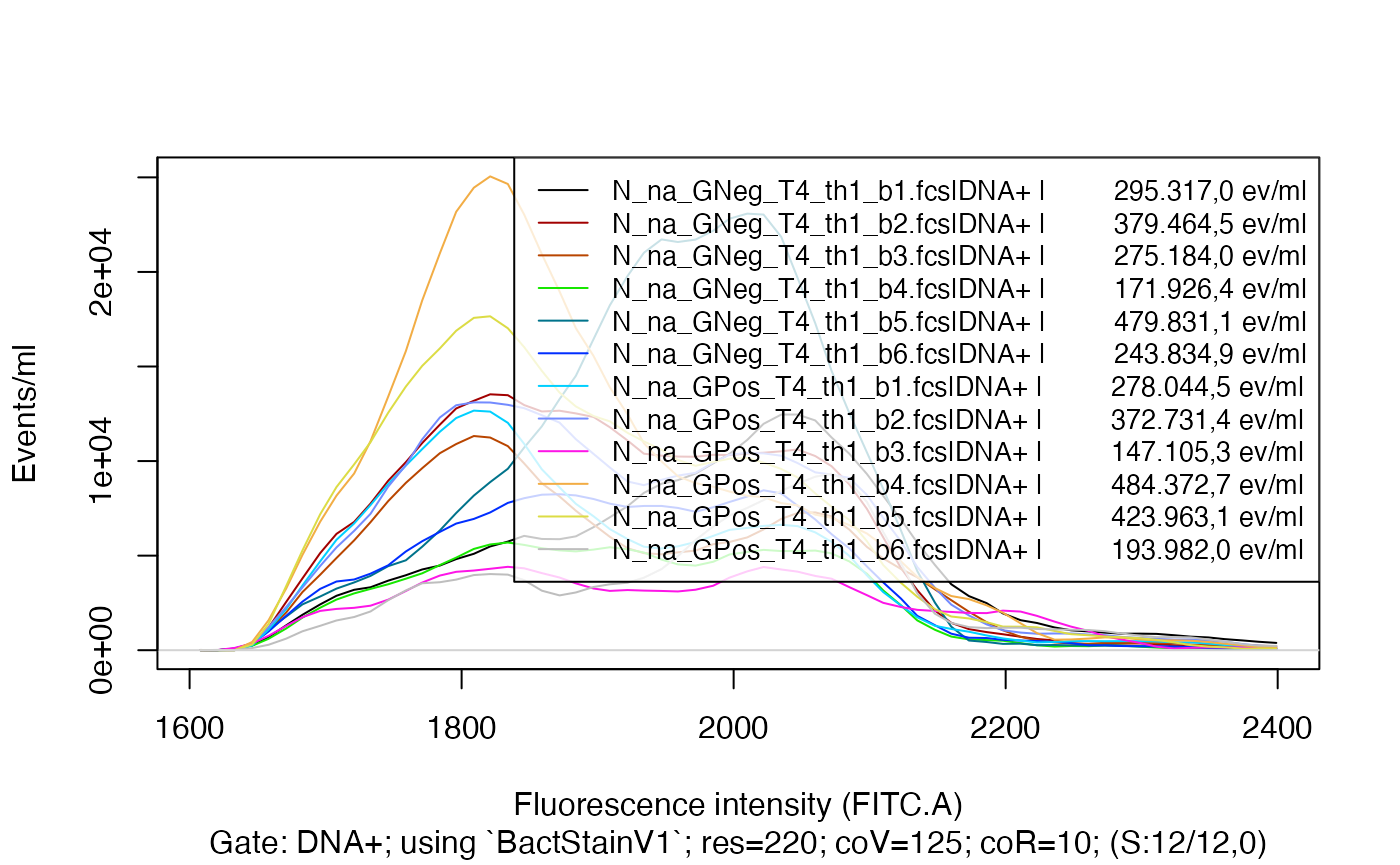
Finally, the rawdata with applied bandpass filter can be exported via
exportFdmatData(fdmat_s_bp, expo.name = "flscData_d4_th1")
#> Exporting data (1 gate) to xlsx...ok.
Enjoy!